Microscopic origin of relaxation
This section illustrates how the microscopic motions observed in a molecular dynamics trajectory give rise to the macroscopic \(^1\mathrm{H}\)-NMR relaxation rates measured experimentally. Using bulk liquid water as a simple example, we follow the complete chain of quantities entering the relaxation calculation, from the motion of individual pairs of nuclei to the dipolar correlation functions and, finally, to the relaxation spectra.
Throughout this section, intramolecular and intermolecular contributions are analysed separately, highlighting how rotational and translational molecular motions contribute differently to NMR relaxation.
MD system
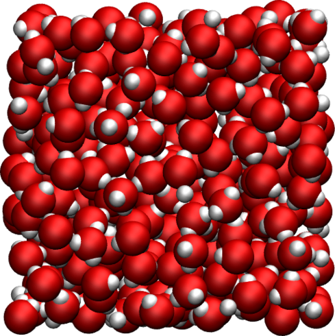
The system is a bulk liquid water with a number \(N\) of water molecules, where \(N\) was varied from 25 to 4000. The simulation box was cubic, with equilibrium dimensions ranging from \((0.9\,\text{nm})^3\) to \((4.9\,\text{nm})^3\). The trajectory was recorded during a \(8\,\text{ns}\) production run performed with the open source codes LAMMPS (for the smallest systems) and GROMACS (for the largest systems). Simulations were performed in the NPT ensemble using a timestep of \(2\,\text{fs}\). The imposed temperature was \(T = 300 \text{K}\), and the pressure \(p = 1\,\text{atm}\). The positions of the atoms were recorded in the prod.xtc file every \(\Delta t\), with \(\Delta t\) ranging from \(0.2\,\text{ps}\) to \(32\,\text{ps}\).
Results
Before analysing the molecular dynamics, we first verify one of the central assumptions used throughout the package. For isotropic bulk liquids, the three second-rank dipolar correlation functions are expected to satisfy [23]
For an isotropic bulk liquid, no direction in space is preferred. The three correlation functions \(G^{(m)}\) differ only by their spherical harmonic order \(m = 0, 1, 2\). Because all orientations are equally probable, the orientation average cannot depend on \(m\), and the functions \(G^{(m)}\) are therefore proportional to one another. The numerical prefactors \(1, 6, 6/4\) arise solely from the explicit forms of the rank-2 spherical harmonics \(Y_2^m\), whose squared moduli satisfy \(|Y_2^0|^2 : |Y_2^1|^2 : |Y_2^2|^2 = 1 : 3 : 3\), combined with the symmetry factor accounting for \(m\) > 0 pairs.
Verifying this proportionality provides a simple consistency check before analysing the relaxation spectra. A similar bencmark was done, for instance in Ref. [15] with glycerol. Our results show that the proportionality relation is well verified (See figure below).
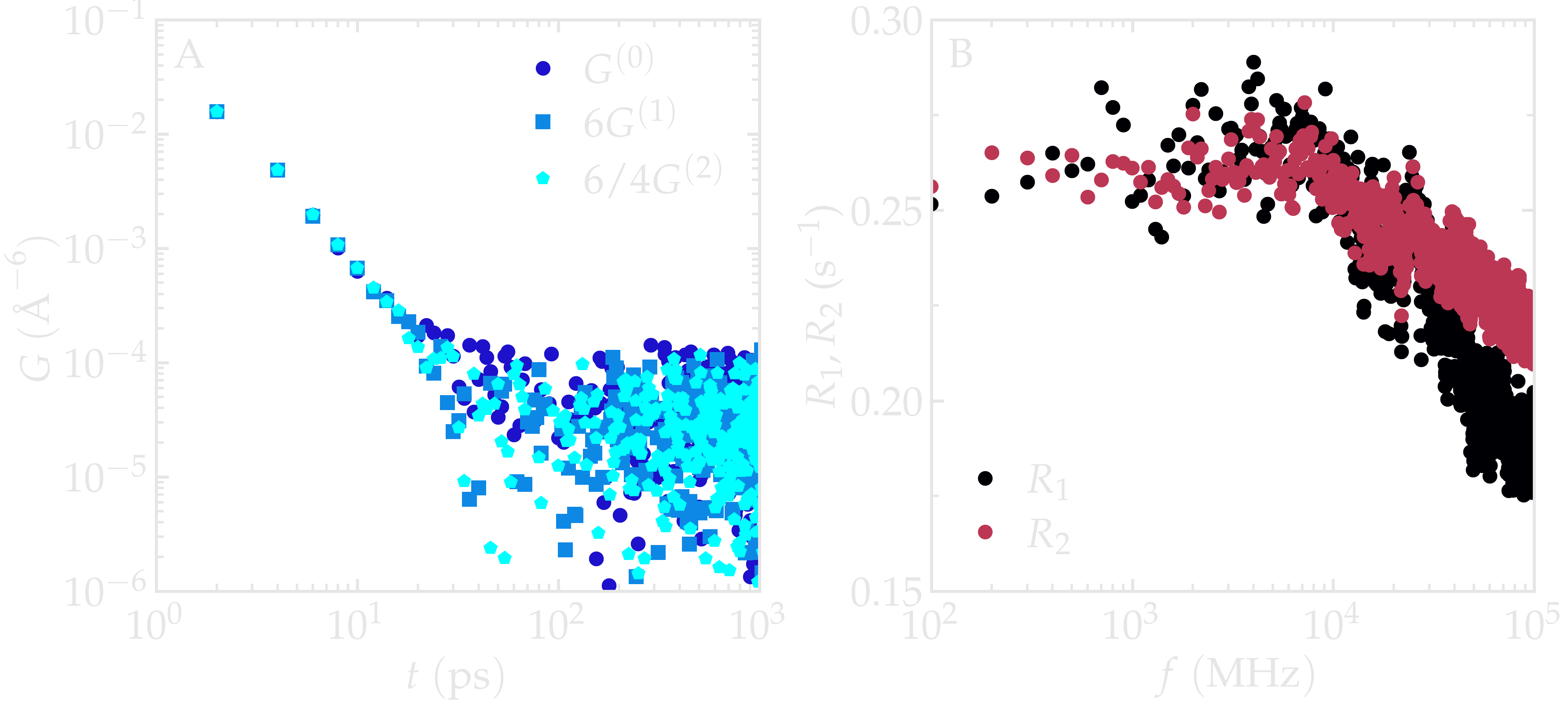
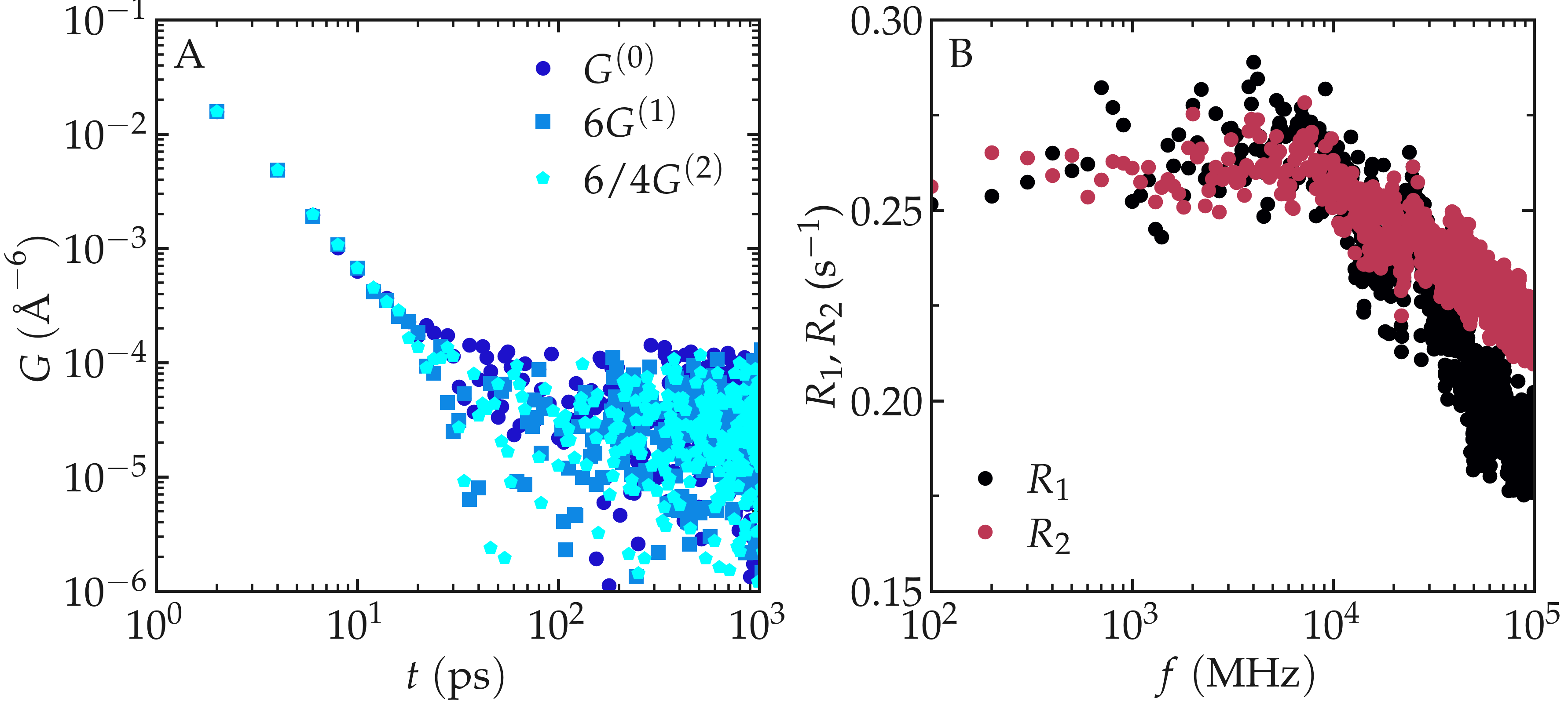
Figure: Test of the validity of the relation \(G^{(0)} = 6 G^{(1)} = \frac{6}{4} G^{(2)}\) on a bulk water system for intramolecular (A) and intermolecular (B) contribution.
Both intra and inter-molecular correlation functions were extracted, and the respective intra and inter NMR spectra were calculated. The total NMR spectrum \(R_1\) was also calculated.
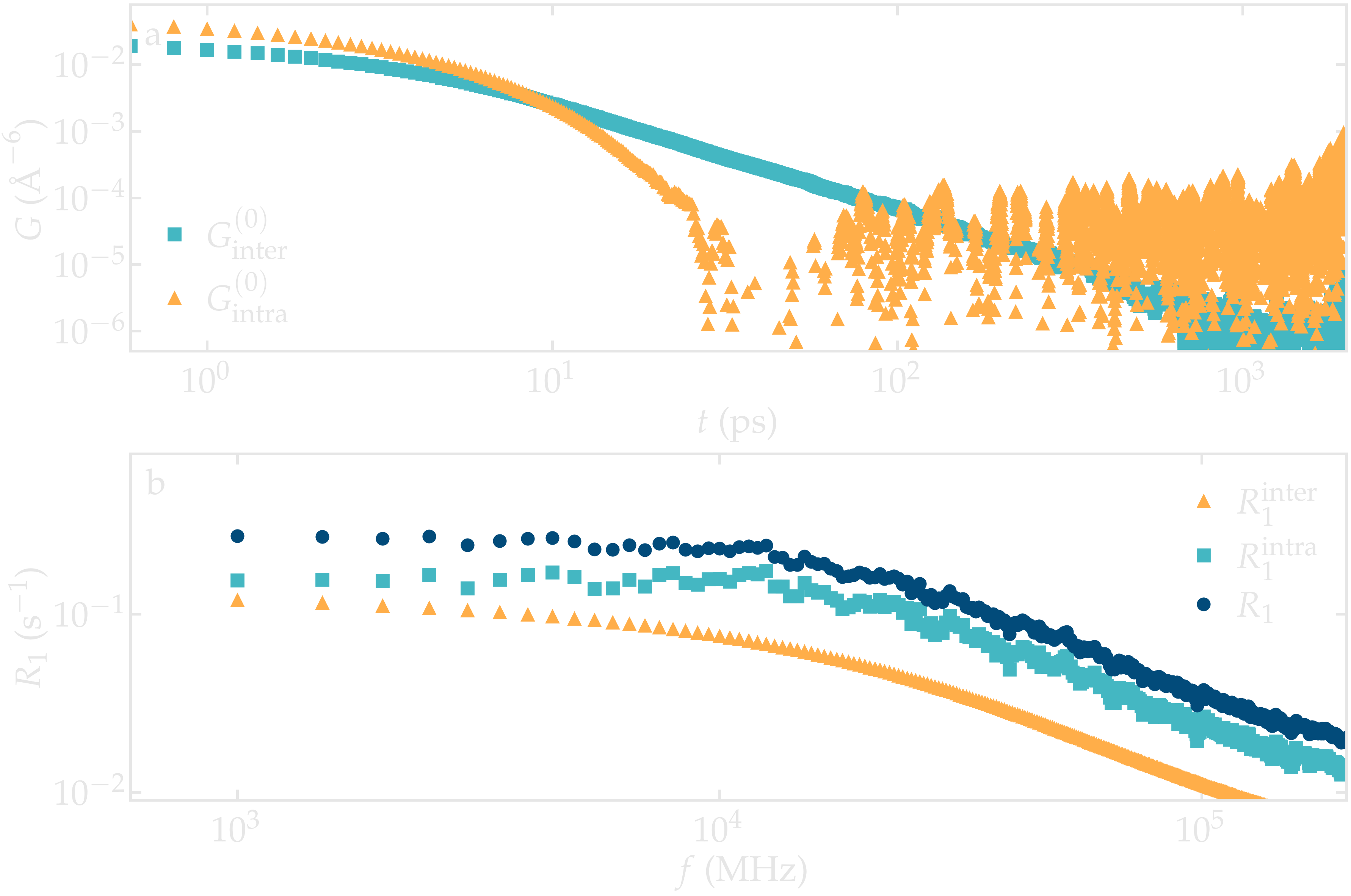
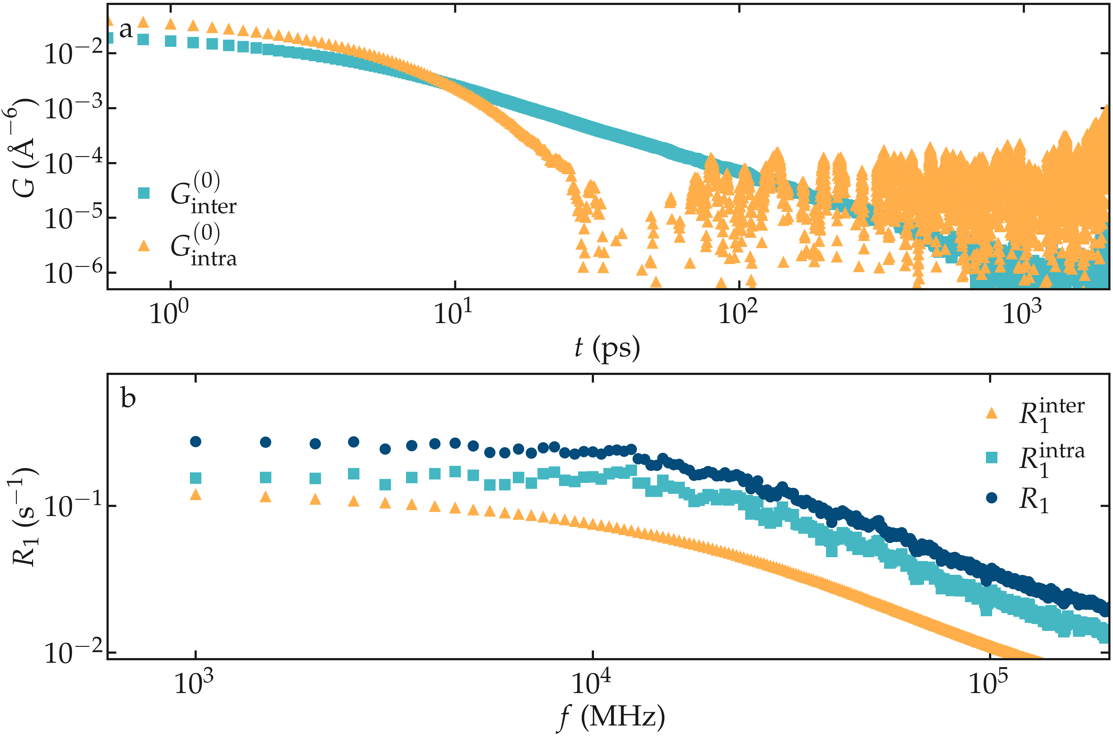
Figure: a) Correlation function \(G^{(0)}\) as extracted from the bulk water simulation with \(N = 4000\) and \(N = \Delta t = 1\,\text{ps}\). b) Corresponding NMR spectra \(R_1\).
The inter-molecular correlation function shows the expected power law at longer time, while the intra-molecular correlation decreases faster with time.
Our results also show that the relaxation is dominated by intra-molecular contribution, as expected for water under ambient conditions [9]. For the lowest frequency considered here, the spectrum \(R_1\) is almost flat.
To understand the origin of these relaxation spectra, it is useful to return to the atomic trajectories themselves. The dipolar interaction between two nuclear spins depends on both their separation \(r_{ij}\) and their relative orientation \(\Omega_{ij}\). Following the evolution of these quantities in time therefore provides direct insight into the microscopic origin of NMR relaxation. Given that the correlations functions are proportional to each others, only \(G^{0}\) and \(J^{0}\) will be evaluated, which depends only in the polar angle \(\theta_{ij}\) as \(Y^{0}_2\) is independent from the azimuthal angle \(\varphi\).
We first consider two hydrogen atoms belonging to the same water molecule. Because the water model is rigid, the internuclear distance remains essentially constant and only the molecular orientation changes with time.
As expected for the rigid water model used here (TIP4P/\(\epsilon\)), the average distance \(r_{ij}\) between the two hydrogen atoms of the same molecule remains constant (within the uncertainty of the shake algorithm used to maintain the water molecule rigid), while the polar angle \(\theta_{ij}\) fluctuates with time, following the rotation of the water molecule (see the Figure below).
The dipolar interaction entering the relaxation equations is described by \(F_2^{(0)}\), which combines the dependence on internuclear distance and orientation. Consequently, even modest rotational motions produce significant fluctuations in \(F_2^{(0)}\).
The fluctuations of \(\theta_{ij}\) with time lead to fluctuations of the function \(F_{0}^{(2)}\) (see Eq. (4)) between a higher bound given by \((3 \cos^2 0 - 1 ) / a^3 \approx 0.58\,A^{-3}\), where \(a \approx 1.51\,A\) is the typical distance between the two hydrogen atoms of the water molecule, and a lower bound \((3 \cos^2 \pi/2 - 1 ) / a^3 \approx -0.29\,\,A^{-3}\).
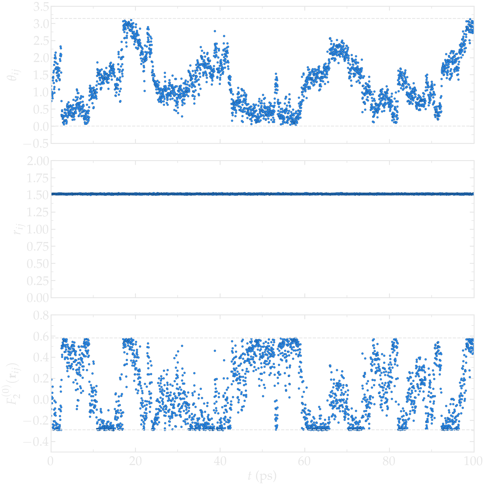
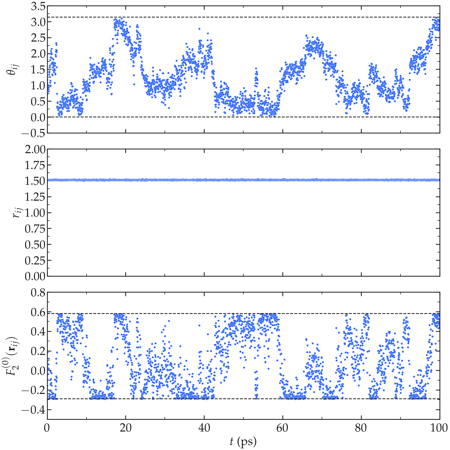
Figure: a) \(\theta_{ij}\) as a function of the time \(t\), where \(i\) and \(j\) refer to two hydrogen atoms located within the same water molecule. a) \(r_{ij}\) as a function of time. c) \(F_{2}^{(0)}\) as a function of time. The temperature is 300 K, and the total number of water molecules is 3000.
We now consider two hydrogen atoms belonging to different water molecules. In contrast with the intramolecular case, both the internuclear distance and the relative orientation fluctuate because of translational diffusion. In that case, \(r_{ij}\) fluctuates significantly between \(\approx 2.5 A\), corresponding to the shortest typical distance between two molecules that are next to one another, to larger values (potentially as large as the box permits). As can be seen, the function \(F_{0}^{(2)}\) reaches its largest absolute values when \(r_{ij}\) is the shorter.
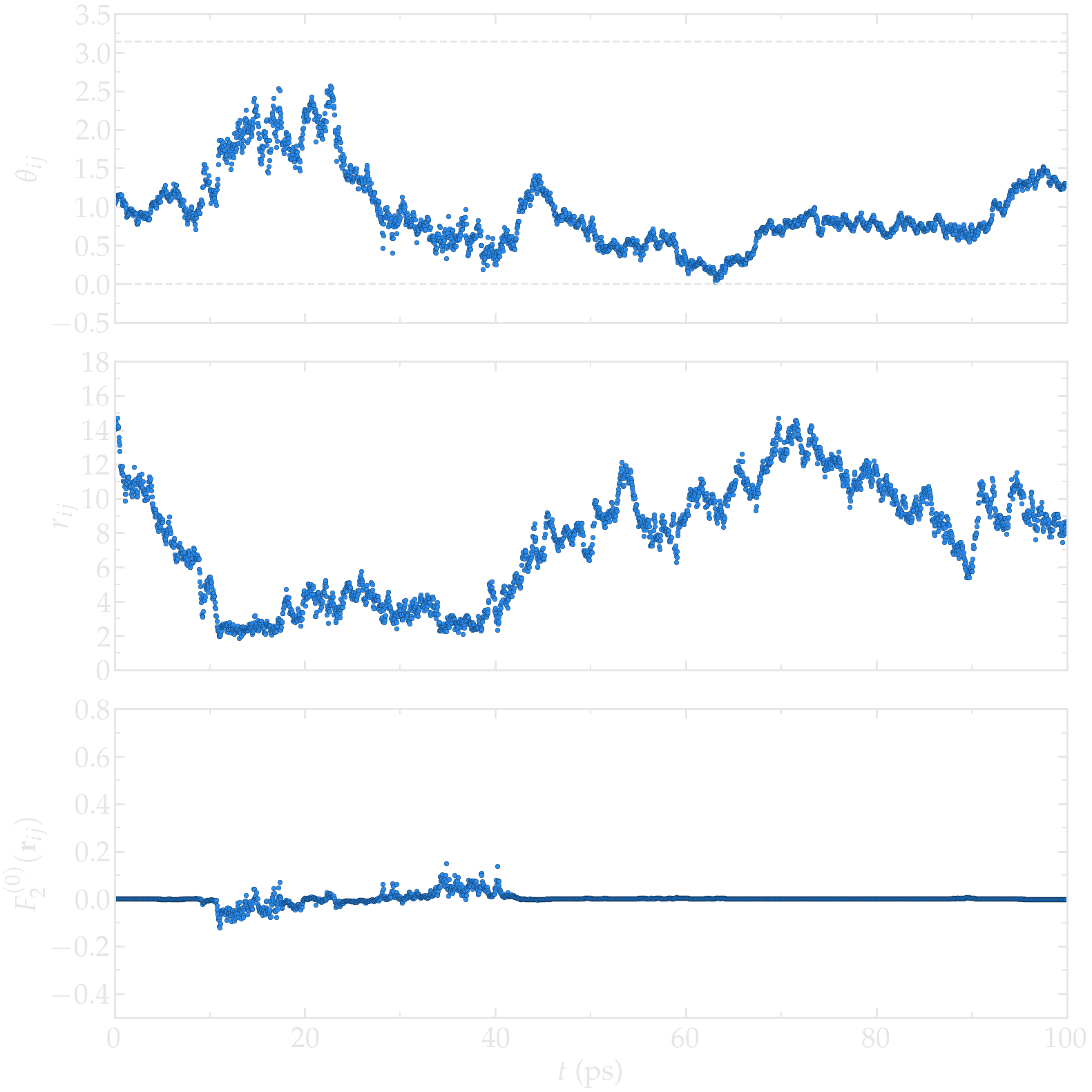
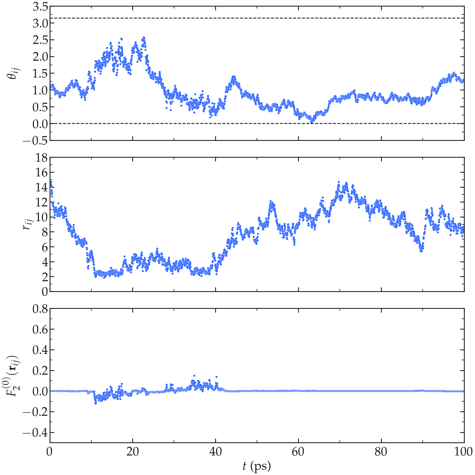
Figure: a) \(\theta_{ij}\) as a function of the time \(t\), where \(i\) and \(j\) refer to two hydrogen atoms located within two different water molecules. a) \(r_{ij}\) as a function of time. c) \(F_{2}^{(0)}\) as a function of time. The temperature is 300 K, and the total number of water molecules is 3000.
Although the behaviour of a single pair of nuclei is informative, NMR relaxation is a collective property. The relaxation rates are obtained by averaging the fluctuations of \(F_2^{(0)}\) over all relevant pairs of nuclei and over the complete molecular dynamics trajectory.
From the fluctuating quantities \(F_{0}^{(2)}\) summed up over all the available pair of spins, one can extract the two correlation functions \(G_\textrm{intra}^{(0)}\) and \(G_\textrm{inter}^{(0)}\) (see Eqs. (2) and (3)). For comparison, the results obtained with two different temperatures 275 and 300 K are reported.
At short time \(t < 40\) ps, the intra-molecular correlation functions follow and a decreasing exponential,
where \(\tau_\text{intra} = 6.3\) ps was used for \(T = 300\) K and \(\tau_\text{intra} = 3.2\) ps was used for \(T = 275\) K, see the figure below. An exponential decay, such as Eq. (1), is common for process governed by a single characteristic correlation time. Such behaviour is commonly used to describe isotropic rotational diffusion and provides a good approximation for the short-time intramolecular dynamics of liquid water [7].
The inter-molecular correlation functions, however, scale as an exponential [i.e. Eq. (1)] only for time shorter than a few tens of pico-second, and show a clear scaling as \(G_\text{inter} (t) \sim t^{-3/2}\) for large time which is a characteristic signature of the diffusion process controlling the motion of the molecules.
At longer times, translational diffusion continually brings new molecular neighbours into and out of the local environment. This diffusive process produces the characteristic long-time \(t^{-3/2}\) decay predicted theoretically for freely diffusing particles. The scaling \(G_\text{inter} (t) \sim t^{-3/2}\) has long been predicted, and analytical expressions have been proposed by Ayant et al. [24] and Hwang and Freed [25], in the context of freely diffusing hard spheres. Following Ref [6], this expression is here referred to as a ADHF.
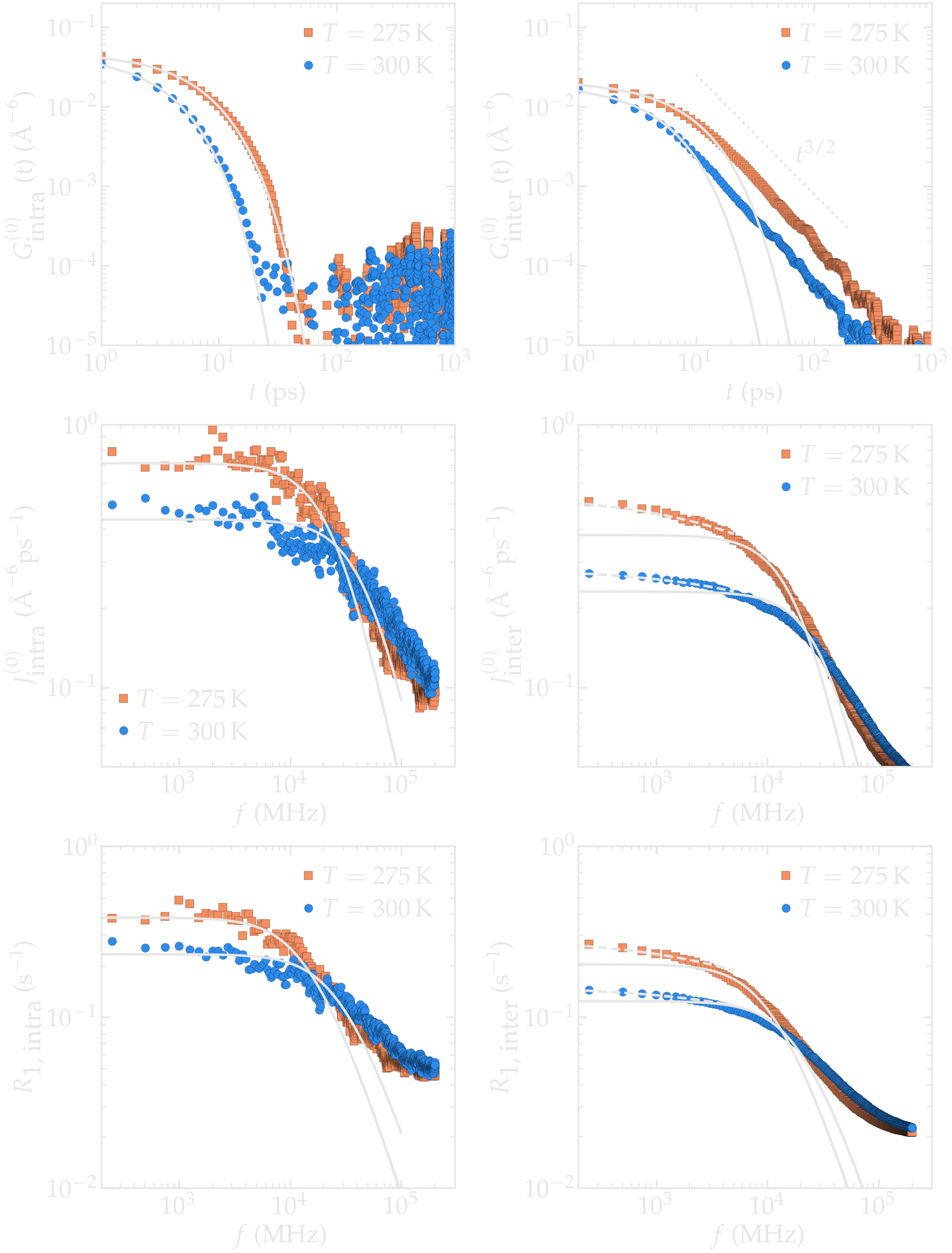
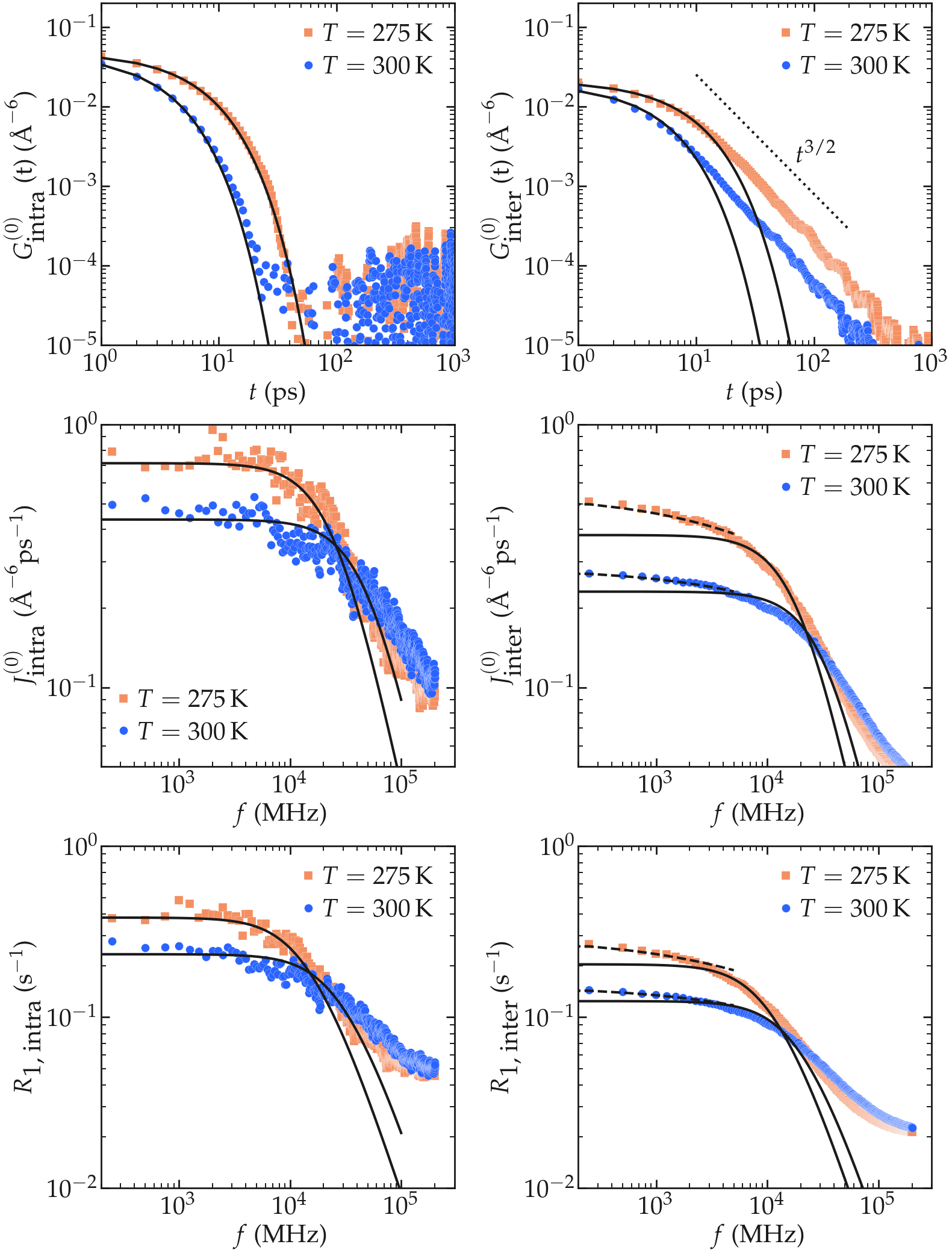
The intra molecular spectrum \(J_\textrm{intra}^{(0)}\) can be reasonably well adjusted by a Lorentzian
using \(\tau_\text{c} = 6.3\) ps and \(G(0) = 56300\) A⁻⁶ ps⁻² for \(T = 300\) K and \(\tau_\text{c} = 3.2\) ps and \(G(0) = 59500\) A⁻⁶ ps⁻² for \(T = 275\) K.
The inter molecular spectrum \(J_\textrm{inter}^{(0)}\), however, does not follow the Lorentzian plateau, particularly at the lowest frequencies, which is consistent with the correlation function \(G_\textrm{inter}^{(0)}\) decaying with time as a power law. In that case, and following closely Ref. [26], an exact analytical expression for the surface spectrum \(J_\textrm{surf} (f)\) can be obtained from the first return passage time of a molecule between successive adsorption and desorption at the surface of a sphere, in the limit of a large diffusing reservoir:
Still from Ref. [26], one can deduce that \(A = k r / D\) and \(B = r / \sqrt{D}\) where \(r\) is here the radius of the water molecule, \(D\) the diffusion coefficient, and \(k\) a phenomenological rate constant with the units of m/s. The frequency scaling as predicted by equation (3) is in good agreement with molecular dynamics results at frequency lower than \(10^4\) MHz.