Isotropic system

Here, we illustrate how the NMRDfromMD package can be applied to a simple MD simulation. The \(^1\text{H}\)-NMR relaxation times \(T_1\) and \(T_2\) are measured from a bulk polymer-water mixture using NMRDfromMD. To follow the tutorial, MDAnalysis, NumPy, and Matplotlib must be installed.

MD system

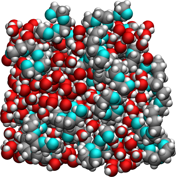
The system consists of a bulk mixture of 420 \(\text{H}_2\text{O}\) water molecules and 30 \(\text{PEG 300}\) polymer molecules. The \(\text{TIP4P}-\epsilon\) is used for the water [22]. \(\text{PEG 300}\) refers to polyethylene glycol chains with a molar mass of \(300~\text{g/mol}\). The trajectory was recorded during a \(10~\text{ns}\) production run performed using the open-source code LAMMPS in the \(NpT\) ensemble with a timestep of \(1~\text{fs}\). The temperature was set to \(T = 300~\text{K}\) and the pressure to \(p = 1~\text{atm}\). Atomic positions were saved in the prod.xtc file every \(2~\text{ps}\).

Note

If you’d like to learn LAMMPS and generate your own trajectories, beginner tutorials are available here [23].

File preparation

To access the LAMMPS input files and pre-computed trajectory data, download the zip archive, or clone the peg-water-mixture dataset repository using:

git clone https://github.com/NMRDfromMD/dataset-peg-water-mixture.git

The necessary trajectory files for this tutorial are located in the data/ directory.

Create a MDAnalysis universe

Open a new Python script or Notebook, and define the path to the data files:

datapath = "mypath/polymer-in-water/data/"

Then, import NumPy, MDAnalysis, and the NMRD module of NMRDfromMD:

import numpy as np
import MDAnalysis as mda
from nmrdfrommd import NMRD

From the trajectory files, create a universe by loading the configuration file and trajectory:

u = mda.Universe(datapath+"production.data",
                 datapath+"production.xtc")

Note

The MDAnalysis universe, u, contains both the topology (atom types, masses, etc.) and the trajectory (atom positions at each frame). These informations are used by NMRDfromMD for the calculation of \(^1\text{H}\)-NMR properties.

Let us print some basic information from the universe, such as the number of molecules (water and PEG):

n_TOT = u.atoms.n_residues
n_H2O = u.select_atoms("type 6 7").n_residues
n_PEG = u.select_atoms("type 1 2 3 4 5").n_residues

print(f"The total number of molecules is {n_TOT} ({n_H2O} H2O, {n_PEG} PEG)")

Executing the script using Python will return:

The total number of molecules is 450 (420 H2O, 30 PEG)

Let us also print information concerning the trajectory, namely the timestep, timestep and the total duration of the simulation, total_time:

timestep = np.int32(u.trajectory.dt)
total_time = np.int32(u.trajectory.totaltime)

print(f"The timestep is {timestep} ps")
print(f"The total simulation time is {total_time//1000} ns")

Executing the script using Python will return:

The timestep is 2 ps
The total simulation time is 10 ns

Note

In the context of MDAnalysis, the timestep refers to the duration between two recorded frames, which is different from the actual timestep of \(1\,\text{fs}\) used in the LAMMPS molecular dynamics simulation.

Launch the \(^1\text{H}\)-NMR analysis

First, we create three atom groups: the hydrogen atoms of the PEG, H_PEG, the hydrogen atoms of the water, H_H2O and all hydrogen atoms, H_ALL:

H_PEG = u.select_atoms("type 3 5")
H_H2O = u.select_atoms("type 7")
H_ALL = H_PEG + H_H2O

Next, we run NMRDfromMD for all hydrogen atoms:

nmr_all = NMRD(
    u=u,
    atom_group=H_ALL,
    neighbor_group = H_ALL,
    number_i=20)
nmr_all.run_analysis()

With number_i = 20, only 20 randomly selected atoms from H_ALL are included in the calculation. Increasing this number improves statistical resolution, while setting number_i = 0 includes all atoms in the group. Here, H_ALL is specified as both the atom_group and the neighbor_group.

Note

In practice, here we don’t have to specify neighbor_group because when it is not specified, atom_group is used instead.

To access the calculated value of the NMR relaxation time \(T_1\) in the limit \(f \to 0\), add the following lines to the Python script:

T1 = np.round(nmr_all.T1, 2)

print(f"The NMR relaxation time is T1 = {T1} s")

The output should be similar to:

The NMR relaxation time is T1 = 1.59 s

The exact value you obtain may differ, as it depends on the specific hydrogen atoms that were randomly selected for the calculation. With the relatively small value for the number of atom taken into account for the calculation, number_i = 20, the uncertainty is significant. Increasing number_i will yield more precise results but at the cost of increased computation time.

Extract the \(^1\text{H}\)-NMR spectra

The relaxation rates \(R_1 (f) = 1/T_1 (f)\) (in units of \(\text{s}^{-1}\)) and \(R_2 (f) = 1/T_2 (f)\) can be extracted for all frequencies \(f\) (in MHz) as nmr_all.R1 and nmr_all.R2, respectively. The corresponding frequencies are stored in nmr_all.f.

R1_spectrum = nmr_all.R1
R2_spectrum = nmr_all.R2
f = nmr_all.f

The spectra \(R_1 (f)\) and \(R_2 (f)\) can then be plotted as a function of \(f\) using pyplot:

from matplotlib import pyplot as plt

# Plot settings
plt.figure(figsize=(8, 5))
plt.loglog(f, R1_spectrum, 'o', label='R1', markersize=5)
plt.loglog(f, R2_spectrum, 's', label='R2', markersize=5)
# Labels and Title
plt.xlabel("Frequency (MHz)", fontsize=12)
plt.ylabel("Relaxation Rates (s⁻¹)", fontsize=12)
# Grid and boundaries
plt.grid(True, which="both", linestyle='--', linewidth=0.7)
plt.xlim(80, 1e5)
plt.ylim(0.05, 2)
# Legend
plt.legend()
plt.tight_layout()
plt.show()

The curves should ressemble the figure below (panel A). For such isotropic systems, one expects \(R_1 (f)\) and \(R_2 (f)\) to have similar values in the limit of low frequency. The same calculation with a much larger value for number_i will lead to much smother curves (see panel B).

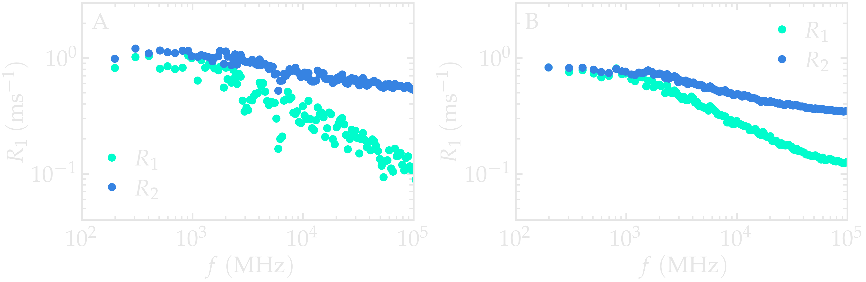
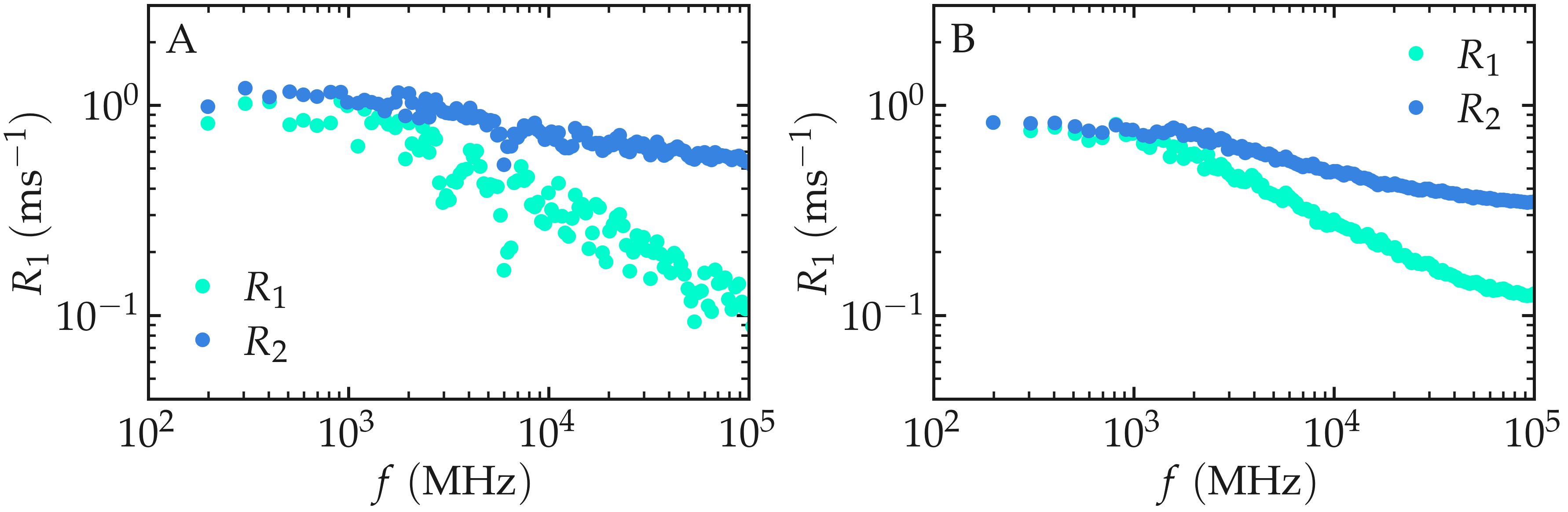
Figure: (A) \(^1\text{H}\)-NMR relaxation rates \(R_1\) and \(R_2\) as a function of the frequency \(f\) for the \(\text{PEG-H}_2\text{O}\) bulk mixture. Results are given for a small value of number_i, \(n_i = 20\). (B) Same quantity as in panel A, but with \(n_i = 1300\).

Separating intra and intermolecular

So far, the calculations were performed for the two molecule types, PEG and \(\text{H}_2\text{O}\), without distinguishing between intra and intermolecular contributions. However, this separation is meaningful and allows for identifying the primary contributors to the relaxation process.

Let us extract the intramolecular contributions to the relaxation for both water and PEG, separately:

nmr_h2o_intra = NMRD(
    u=u,
    atom_group=H_H2O,
    type_analysis="intra_molecular",
    number_i=200)
nmr_h2o_intra.run_analysis()

nmr_peg_intra = NMRD(
    u=u,
    atom_group=H_PEG,
    type_analysis="intra_molecular",
    number_i=200)
nmr_peg_intra.run_analysis()

We can also measure the intermolecular contributions:

nmr_h2o_inter = NMRD(
    u=u,
    atom_group=H_H2O,
    type_analysis="inter_molecular",
    number_i=200)
nmr_h2o_inter.run_analysis()

nmr_peg_inter = NMRD(
    u=u,
    atom_group=H_PEG,
    type_analysis="inter_molecular",
    number_i=200)
nmr_peg_inter.run_analysis()

Importantly, when no neighbor_group is specified, the atom_group is used as the neighbor group. Thus, in this case, intermolecular contributions are calculated between molecules of the same type only.

When comparing the \(^1\text{H}\)-NMR spectra nmr_h2o_inter.R1 and nmr_h2o_intra.R1, you may observe that the intramolecular contributions to \(R_1\) are larger than the intermolecular contributions. Additionally, the intra- and intermolecular spectra display different scaling with frequency \(f\), reflecting distinct motion types contributing to each term.

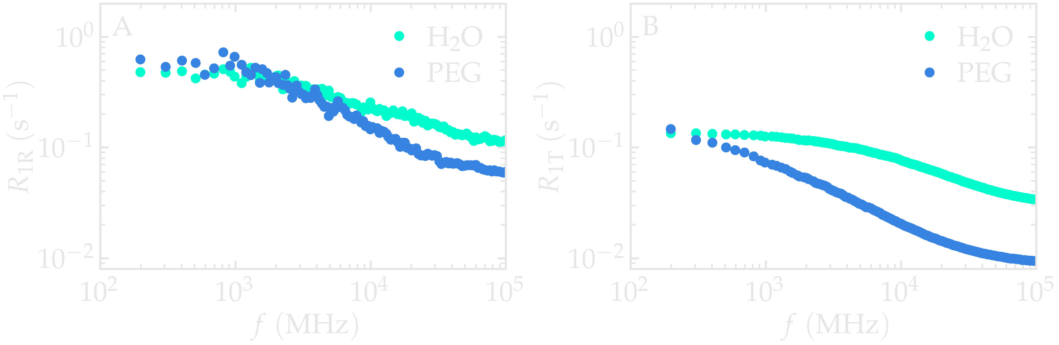
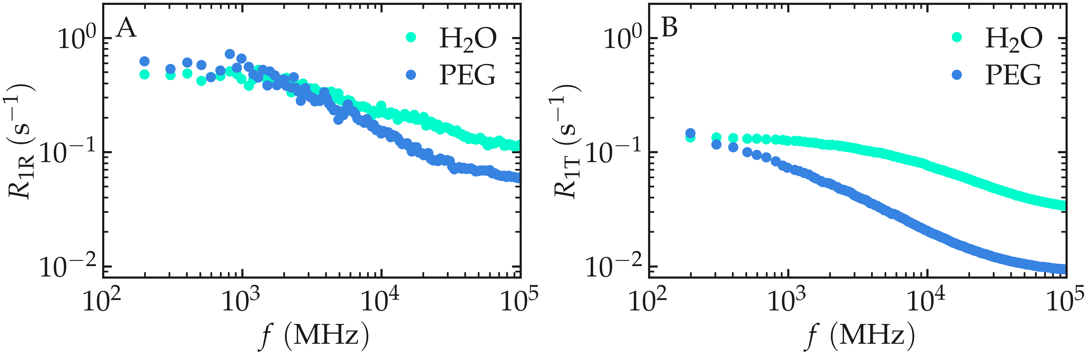
Figure: Intramolecular \(^1\text{H}\)-NMR relaxation rates \(R_{1 \text{R}}\) (A) and Intermolecular \(^1\text{H}\)-NMR relaxation rates \(R_{1 \text{T}}\) (B) as a function of the frequency \(f\) for PEG and \(\text{H}_2\text{O}\) separately. Results are shown for \(n_i = 1280\).